![]()
LBE Tutorial Exercise 1: Single component LBE simulations
We are going to work with a simple two-dimensional LBE code written in C, CCP5_01.c, which applies single-relaxation-time Bhatnagar-Gross-Krook (BGK) collisions, i.e. LBE with BGK or LBGK. This code will carry out LBE over a certain number of timesteps and write out files with results for the final calculation timestep.
The data_density.csv and data_density.dat files print the fluid density \(\rho (x, y)\) at each grid point, while the data_stfn.csv and data_stfn.dat files print a scalar stream function, \(\psi (x, y)\), which can be used to plot lines where flow speeds are constant. (More details about stream functions can be found in our Outline Notes on Fluid Mechanics.) The two sets of files are in different formats: the
files with comma-separated values (CSV) can be read into spreadsheet programs or used with our Python plotting scripts, while the other files are formatted using fixed-length delimiting and can be read into e.g. Gnuplot.
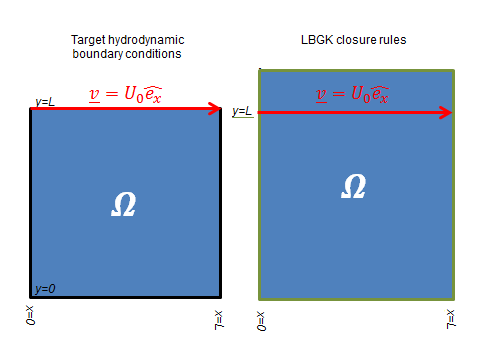
The system we are modelling with this code - 2D flow inside a square ‘lid-driven’ cavity (illustrated in Figure 1) - is described in more detail here. We are going to ask you to make some modifications to this code for some of the exercises: if you are not entirely familiar with C, we have some hints on how to make modifications to codes written in this language in our introduction to the Mesoscale Exercises.
 |
|- -:
Figure 1: Target hydrodynamic boundary conditions (left) and the corresponding LBE lattice closure rules (right) to be used throughout this LBE Tutorial Exercise to represent a ‘lid-driven cavity’ system. The black lines denoting the hydrodynamic boundary condition \(\mathbf{v} = \mathbf{0}\) (left) are represented by bounce-back closures in LBE simulations (right, green lines), while the red lines denote fluid assumed to be moving at velocity \(U_0 \mathbf{\hat{e}}_x\).
Ex1. Code familiarisation/concepts from theoretical fluid mechanics
Start by taking a look through CCP5_01.c, before compiling it using the following command:
[ ]:
!gcc -o LBE CCP5_01.c
This should generate an executable called LBE which can be launched at a command-line:
./LBE N
where N is the required number of timesteps: if no value is supplied, a default value of 4000 is used. The code will carry out LBE calculations over this number of timesteps and print each timestep number to the screen. To avoid producing a long stream of numbers, we have a Python script available to launch the calculation and collect those numbers in a scratch file (which we will delete afterwards), using these to keep track and display a progress bar:
[ ]:
from launchlbe import *
run_LBE('LBE', 4000, '')
Once the calculation is complete, visualise the results using the following script:
[ ]:
from plotlbe import *
plotLBE('data_density.csv', 'Density plots', False)
plotLBE('data_stfn.csv', 'Stream function plots', True)
Checks
Is the observed flow pattern from the stream function plot what you expected?
Stability
Calculate the current Reynolds number \(Re = UL / \nu\) for the flow. Use the lid velocity (
UXin the code) as the characteristic velocity \(U\), the system height (excluding the discarded section,YLENGTH_SYS) as the characteristic length \(L\), and get hold of the kinematic viscosity from the relaxation frequency \(\omega\) (set in the code asOMEGA) and this equation given in your lecture notes:
Now try changing the simulation lid velocity and run the simulation again, remembering to re-compile the code each time. We believe the simulation should be stable for \(Re<200\) or so, but this stability will depend on how you achieve a particular Reynolds number. Verify this fact by carrying out a few experiments.
Reynolds’ number variation
Observe results for Reynolds numbers from 10 to 100. Note that the boundary conditions installed in our code are robust and simple, but not terribly accurate (sorry!).
Using what you have learned about the stability of our code, record and plot approximate spatial locations of the centre of the primary vortex as functions of \(Re\). You can do this by identifying the maximum absolute value of the stream function \(\psi\). We have a script prepared to help you do just that:
[ ]:
from plotlbe import *
findVortex('data_stfn.csv')
Dynamic similarity
Obtain and save stream function data for e.g. \(Re = 50\) for the lid-driven cavity.
Double both the system size and the simulation’s kinematic viscosity \(\nu\) (related to the LBGK relaxation parameter \(\omega\)) so \(Re\) will not change before running the simulation again, and compare the stream function contours with those of the original system size.
You should find that while the numerical values of \(\psi\) will differ, the shapes of the two streams should be pretty much identical. Given these steady-flow simulations have the same value of \(Re\), they are ‘dynamically similar’ and can be related to each other by simple scale transformation.
Time-marching and steady-state flow
Revert to the original version of CCP5_01.c with its original parameters. Hint: For this and other exercises, you might want to keep a copy of this original code somewhere safe in case you want to go back to it later.
Keeping \(Re\) fixed, change the number of LBE calculation steps (
T) and observe the stream function at regular intervals to observe how the flow progresses to a steady state.Every cycle of a LBE simulation corresponds to an evolution of simulated flow over a small time interval \(\Delta t\), and each timestep produces a solution of the Navier-Stokes and continuity equations. LBE is therefore a time-marching method: it cannot ‘directly’ calculate a steady state (unlike some CFD solvers), but must compute all intervening states of the flow field.
Ex2. Manipulation of boundary conditions for complex flow
Modify the code to use mid-link bounce-back boundary conditions instead of on-link ones. Hint: Comment out the currently-used lines in
DirichletBoundaryApply1()for on-node bounce-back and uncomment the ones for mid-link calculations.
One of LBE’s main strengths is its ability to incorporate geometrically complicated boundary conditions rather easily, certainly compared with traditional CFD methods.
Set a Dirichlet boundary condition in the code to represent a submerged jet at the centre of the cavity: we want to set a density and velocity of your choice at a given point, so try applying equilibrium forcing in a similar way to the lid.
Observe what happens to the stream function as a result.
Ex3. Computational Efficiency
When looking at how efficiently a code such as CCP5_01.c runs, our first place to look for time savings will be computational operations that are repeated at every lattice point and during every timestep. These can include calculations of observables (density, velocity, streaming functions) and collisions, which are demanding operations for LBE.
We know that our
Collide()function is pretty inefficient, so try re-writing this function to make the collisions go faster. Hint: Rather than making calls to other functions, try ‘in-lining’ code in this function.Only if you have time, consider how you might improve the efficiency of the
Calc_obs()function.
Remark: A code such as DL_MESO_LBE, which is a repository of several different LBE geometries (lattices) and sub-algorithms, is heavily optimised exactly along these lines, as well as some others for propagation (another time-consuming step). One caveat (or maybe two!): heavily optimised code can be (i) impossible to read (we speak from weary experience) and (ii) hard to modify.
Ex4. A fix for incompressible Navier-Stokes’ fluids
Warning: This is quite a tricky exercise for less experienced coders, so please feel free to skip this exercise (and go on to Ex5) unless you have the time and patience.
Given that the usual form of LBE is mildly compressible, this can introduce errors when modelling flows of incompressible fluids (particularly liquids). Fortunately, there is an exactly incompressible LBGK (‘EILBGK’) method we can develop and apply in our code. This involves a change to the definitions of the local equilibrium distribution function:
and the macroscopic velocity:
where \(\rho_0\) in both cases is the initial (constant) density set in the simulation.
Revert back to the original form of CCP5_01.c.
Modify the equilibrium distribution function to simulate an incompressible fluid at steady-state, i.e. $ f_i^{(0)}$ given above, and the definition of the macroscopic velocity \(\mathbf{u}\).
Confirm your code runs and produces stable results, and observe what you get. Bear in mind that the (variable) density is now re-interpreted as the fluid pressure, i.e. \(\rho = p = \sum_i f_i\), while the fluid density is constant.
Due to the above changes, the EILBGK model is strictly only valid for steady flows, although it is still pretty accurate even in the presence of time variations. This ‘fix’ to LBGK’s weakly compressible form of the Navier-Stokes equations does away with compressibility errors for simulations at steady state.
A solution for this exercise, EILBGK.c, is available to take a look at and try out. (Note the change in file name and contents for the pressure rather than the density!)
[ ]:
from launchlbe import *
from plotlbe import *
!gcc -o EILBGK EILBGK.c
run_LBE('EILBGK', 4000, '')
plotLBE('data_pressure.csv', 'Pressure plots', False)
plotLBE('data_stfn.csv', 'Stream function plots', True)
findVortex('data_stfn.csv')
Ex5. The viscous stress tensor
We now want to look at another observable property, the viscous stress tensor \(\sigma^{\prime}_{\alpha\beta}\), which we can calculate for each lattice point using the following expression:
Note that this property could otherwise be calculated using velocity gradients (see our notes in fluid mechanics), which in conventional CFD methods have to be evaluated by costly non-local calculations. However, in LBE the viscous stress and full stress are available locally without calculating gradients. This is a notable advantage of LBE, ‘locality of stress information’, and can be exploited for modelling non-Newtonian fluids, whose viscosities vary according to local strain rates and can be set as local relaxation times or frequencies.
Another point related to our lid-driven cavity flow: the results of stress calculations may be surprising, given that much of the cavity flow in its bulk approximates potential flow (inviscid flow with negligible viscous stressts).
Revert back (again) to the original CCP5_01.c code.
Add in calculations of \(\sigma^{\prime}_{\alpha\beta}\) for all possible permutations, noting that \(\alpha\) and \(\beta\) can be \(x\) or \(y\). Since these are only needed at the end of a calculation, we suggest creating a separate function similar to
calc_obs()to call once the calculations are complete and outputting the results by modifyingReport(). (Hint: the off-diagonal terms \(\sigma^{\prime}_{xy}\) and \(\sigma^{\prime}_{yx}\) are functionally identical based on the above definition, so you only need to calculate one of these!)
A solution for this exercise, sigma.c, is available to take a look at and try out. Note that it currently only writes out the ‘off-diagonal’ term \(\sigma^{\prime}_{xy}\), but you will be able to use the above plotting script to visualise it.
[ ]:
from launchlbe import *
from plotlbe import *
!gcc -o sigma sigma.c
run_LBE('sigma', 4000, '')
plotLBE('data_density.csv', 'Density plots', False)
plotLBE('data_stfn.csv', 'Stream function plots', True)
plotLBE('data_stress_xy.csv', 'xy-component of viscous stress tensor', False)