LBE Tutorial Exercise 2: Multi-Component LBE simulations¶

Code transformation¶

The real interest in MCLB applications is in their dynamics; we want to simulate e.g. immiscible fluids interacting with each other. Imagine an oil drop in water. If the ‘external’ fluid (water here) moves, it exerts stresses on the surface of the oil and causes it to move, while the interior fluid (oil) impedes the motion of the water: action and reaction and all that. The resulting dynamics are complex: given the interface (with its own physics, as you can see in Ex1 in the previous notebook) deforms, re-locates the boundary between fluids, modifies the interaction … hopefully you get the point! With MCLB, all of these physics are in place as you hopefully saw in CCP5_02.c … we will now try and convince you by switching to a more comprehensive LBE code.

DL_MESO_LBE, the LBE code in DL_MESO, is an ideal tool to observe complex, multi-component hydrodynamics. It can work in 3D but we will stick to 2D to allow fast computation and interaction/experimentation. In the last set of exercises, we shall configure and use DL_MESO_LBE to perform simulations of a neutrally buoyant drop of red fluid (oil) suspended in a blue fluid (water), which is moved at its boundaries to produce a shear flow (as seen in Figure 1 below).

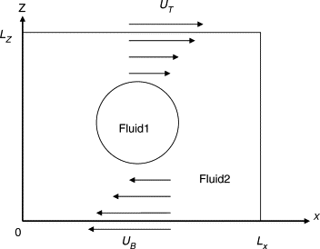
Boundary conditions for sheared drop system

-:

Figure 1: Schematic of a sheared drop (Fluid1). Flow is applied to the boundaries of the external fluid (Fluid2) and the fluid motion is communicated throughout the domain, mainly by viscous forces.

We shall perform some experiments using DL_MESO_LBE - which we can view using scripts and ParaView - allowing us to observe the hydrodynamics of the system, both in terms of the change in the drop’s shape and the complex flow patterns that arise.

Ex4. Equilibration dynamics with DL_MESO_LBE¶

We have supplied a ZIP file with the source code for both of DL_MESO’s codes. Unpack this ZIP file using the command:

[ ]:

!unzip -o -q ../Day_9Meso/dl_meso_2.7.zip

and then go into its dl_meso/WORK directory and compile DL_MESO_LBE for a single processor core with OpenMP multithreading (to speed up the calculations) using the following:

[ ]:

%%bash
cd dl_meso/WORK
g++ -o lbe.exe -O3 -fopenmp ../LBE/slbe.cpp

This provides an executable file for DL_MESO_LBE (lbe.exe) that we can use to run a simulation, provided we have the required input files.

The input files for our sheared drop calculation are in the LBE2Ex4 directory: lbin.sys provides simulation system controls (including values for \(\alpha\) and boundary velocities), lbin.spa specifies boundary conditions and lbin.init provides an initial state, which adds a drop of fluid 1 (our ‘red’ fluid) with a radius of 10 right in the middles of fluid 0 (our bulk ‘blue’ fluid). To launch the calculation, either use the following commands (ideally in a terminal window):

[ ]:

%%bash
cd LBE2Ex4
export OMP_NUM_THREADS=6
../dl_meso/WORK/lbe.exe

or the following script to launch DL_MESO_LBE in the specified folder and keep track of its progress.

[ ]:

import os
import launchdlmeso as dlm
os.environ["OMP_NUM_THREADS"] = "6"
dlm.run_LBE('LBE2Ex4', 'dl_meso/WORK/lbe.exe', 1, True, '')

Note that we are setting the number of OpenMP threads in the commands just before launching DL_MESO_LBE. While it might be tempting to use all (16) available threads, overheads involved in splitting sections of the calculation can actually slow things down, so a balance is required. We recommend using just under half of the available threads (i.e. 6).

DL_MESO_LBE will print a summary of the calculation either to the screen (if running in a terminal window) or to a file (if using the script), and generate a series of structured grid VTK files (e.g. lbout000000.vts) after an equilibration period of 5000 timesteps to allow the drop to settle first. These files are snapshots of the simulation that can be opened and visualised in ParaView. (We also have some Python scripts to look at these.)

Take a look at the simulation output files. If you are using ParaView, you should be able to generate animations of e.g. drop fluid density. The Calculation filter can be used to find properties derived from those supplied in the files, e.g. total fluid densities \(\rho\) can be calculated using:

density_0+density_1

and phase indices \(\rho^N\) using:

(density_1-density_0)/(density_0+density_1)

as expressions in the Calculation filter. The Contour filter can be used on phase indices to find the centre of the interface between the two fluids (i.e. where \(\rho^N = 0\)) and plot the drop shape.

Alternatively, we can use the following script to read in a specific output file and plot the total densities, phase indices and velocity (both the modulus and the x- and y-components), as well as show the interface between the fluids in the velocity plots as a black line.

[ ]:

from plotvtk import *
plotVTK('LBE2Ex4/lbout000200.vts')

What happens to the drop when the shearing boundaries (at the top and bottom of the domain) are applied?

The lbin.sys file consists of keywords that allow you to change operating parameters for the calculation. The most relevant keywords for this exercise are:

speed_top_0 - the x-component of velocity for the boundary at the top of the domain
speed_bot_0 - the x-component of velocity for the boundary at the bottom of the domain
interaction_0_1 - the interaction parameter (interfacial tension \(\alpha\)) between fluids 0 (blue) and 1 (red)
segregation - the segregation parameter \(\beta\) used to ‘recolour’ the fluids after collisions
interaction_type - the MCLB algorithm we want to use, currently set to Lishchuk (the name of the algorithm in DL_MESO_LBE)

Note that the value of \(\beta\) we are using in DL_MESO_LBE is around double the value we used in CCP5_02.c. This is due to a slight difference in how segregation is carried out between the two codes, although the general trends regarding interfacial width and stability will be similar.

Try changing the wall velocities and/or the interfacial tension between the fluids. What happens if the shear rate decreases or the interfacial tension increases (i.e. \(Ca\) decreases)?
What happens if you increase \(Ca\) (increase shear rate or decrease interfacial tension)?
Can you find a minimum value of \(Ca\) at which the drop starts to break up due to the flow?

The very first output file (lbout000000.vts) is written immediately after equilibration and should provide a good representation of a static drop. Try visualising the drop with this file and use the following script to find a few related properties.

[ ]:

from plotvtk import *
findCOMradius('LBE2Ex4/lbout000000.vts')

Take a look at the velocity field: where are the maximum velocities in relation to the drop’s location?
What happens to these microcurrents when you vary \(Ca\)?

Ex5. DL_MESO code modification¶

As well as a complete LBE code with a wide range of collision and fluid/phase models, DL_MESO also provides its subroutines for users to come up with custom codes of their own to test new functionalities and possibly improve computational performance.

We have devised a couple of custom codes to implement our MCLB algorithm (known as the ‘Lishchuk method’ in DL_MESO_LBE) in a couple of different ways:

slbe-lishchuk.cpp implements the standard form of the algorithm, which calculates interfacial normals \(\mathbf{n}\), interfacial curvatures \(K\) and the following forces between fluids (implemented in collisions using Guo’s forcing term):

\[\mathbf{F} = \frac{1}{2} \alpha K \nabla \rho^N\]

slbe-spencertensor.cpp implements a variant algorithm, known as ‘Spencer tensor’, which replaces the interfacial curvature and force calculations with a special forcing term added to collisions:

\[F_i = \frac{t_i \beta \alpha \omega \rho_0 \rho_1}{c_s^4 \rho^3 \Delta t} \left(\mathbf{nn} - \mathbf{I}\right) : \left(\mathbf{c}_i \mathbf{c}_i - c_s^2 \mathbf{I} \right)\]

Use the following commands to copy the custom codes into the dl_meso/LBE directory and then compile both codes in turn.

[ ]:

%%bash
cp LBE2Ex5/*.cpp dl_meso/LBE
cd dl_meso/WORK
g++ -o lbe-lishchuk.exe -O3 -fopenmp ../LBE/slbe-lishchuk.cpp
g++ -o lbe-spencertensor.exe -O3 -fopenmp ../LBE/slbe-spencertensor.cpp

The resulting executables can be run in the same manner as DL_MESO_LBE above, using the newly-created executable files (dl_meso/WORK/lbe-lishchuk.exe and dl_meso/WORK/lbe-spencertensor.exe) instead of dl_meso/WORK/lbe.exe, but with the same input files, e.g.

[ ]:

import os
import launchdlmeso as dlm
os.environ["OMP_NUM_THREADS"] = "6"
dlm.run_LBE('LBE2Ex4', 'dl_meso/WORK/lbe-lishchuk.exe', 1, True, '')

Try out lbe-lishchuk.exe with the previous exercise’s input files. You should get identical results compared with DL_MESO_LBE: do you observe any noticeable speedup?
Try out lbe-spencertensor.exe with the same input files. Do you get similar results? How do the microcurrents during equilibration compare between the two codes?

One advantage of the implementation of the Lishchuk MCLB algorithm in DL_MESO_LBE is we can extend it to more than two fluids, meaning we could have more than one drop in a background fluid. We can define different phase indices for the drops (with the background fluid and each other) and associated interfacial normals, determine curvatures between the fluids where they interact and calculate forces between each pair of fluids … or work out forcing terms for our ‘Spencer tensor’ implementation.

We have a system available with three fluids - a background fluid (0) and two immiscible drops (fluids 1 and 2) - available in the LBE2Ex5 directory: lbin.sys, lbin.spa and lbin.init. This is similar to the one from the previous exercise, in that we are subjecting the system to linear shear, but we have ‘accidentally’ (on purpose) put the two drops in at the start so they partially overlap each other. We are confident that the MCLB’s segregation step will manage to separate out the drops. (Famous last words!)

Set the calculation going for this system using each of the two custom codes with the script below or the default version of DL_MESO_LBE: if you want to use the latter, change the interaction_type in lbin.sys to LishchukSpencerTensor to use the ‘Spencer tensor’ algorithm.

[ ]:

import os
import launchdlmeso as dlm
os.environ["OMP_NUM_THREADS"] = "6"
dlm.run_LBE('LBE2Ex5', 'dl_meso/WORK/lbe-lishchuk.exe', 1, True, '')

Once each version of the calculation has finished, visualise their results either by using ParaView or the scripts provided below. Note that we can define the phase index for the second drop using the following expression in ParaView’s Calculation filter:

(density_2-density_0)/(density_0+density_2)

although you may find for one of the cases that this expression on its own (and the similar one for the first drop) might not be enough to find the boundary between two conjoined drops. To get around this, we suggest adding a condition for each phase index to test how much the background and drop fluids contribute to the total density at a given lattice point, which we can do with an if statement in the expression for the Calculation filter, e.g.

if((density_0+density_2)/(density_0+density_1+density_2)>0.5, (density_2-density_0)/(density_0+density_2), -1.0)

[ ]:

from plotvtk import *
plotVTK('LBE2Ex5/lbout000200.vts')
findCOMradius('LBE2Ex5/lbout000200.vts')

What happens to the drops immediately after equilibration and during the simulation for both versions of the code (or both algorithms)?
Can you think why the two versions of the MCLB algorithm behave differently in this case? (Hint: how can a curvature between more than two fluids be calculated?)

Try extending the number of timesteps in the simulation by increasing the number given with total_step in the lbin.sys file, or try increasing the speeds of the top and bottom boundaries to increase the shear rate.

What happens when two moving drops collide into each other? How would or could you control that process? (Hint: Take a look in the lbin.sys file.)