DPD Tutorial Exercise 2: Applying DPD to molecular systems¶

Ex1. DPD mesophases¶

We are now going to extend our DPD calculations from those in the previous exercise to include additional interactions between some particles and form mesoscopic representations of molecules. This vastly extends the range of systems DPD can model, which is well-suited to finding larger scale structures relatively quickly (compared with atomistic MD).

The simplest molecular structures we can create are dimers, molecules consisting of two beads joined together with a bond (e.g. a harmonic spring). If the dimer is amphiphilic, the two beads interact differently with solvent beads; the hydrophobic beads repel solvent beads more strongly, while hydrophilic beads have stronger affinity for the solvent (or repel each other less strongly).

The concentration of amphiphilic molecules in solution and temperature have an effect on the structures the molecules can form. Our dimers can produce one of three distinctive phases:

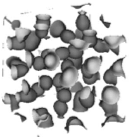
• Isotropic phases with spherical ‘blobs’ of material

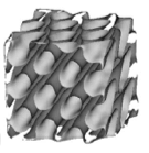
• Hexagonal phases of long tubes laid out in hexagonal patterns

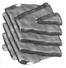
• Lamellar phases of parallel ‘sheets’ (lamellae)

In this exercise, we have four DL_MESO_DPD simulations of amphilphilic dimers we can run, visualise and analyse. If you have not yet already done so, make sure you have compiled DL_MESO_DPD - first by unzipping the ZIP file:

[ ]:

!unzip -o -q dl_meso_2.7.zip

and then invoking the required (OpenMP) makefile:

[ ]:

%%bash
cd dl_meso/WORK
make -f Makefile-OMP clean
make -f Makefile-OMP

The four simulations are available in folders inside the DPD2Ex1 directory. Each consists of a CONTROL file - the same for each simulation - and a FIELD file that defines three bead types (S = solvent, A = hydrophilic bead, B = hydrophobic bead) and the topology of our amphiphlic dimers (AB). The FIELD files differ by concentrations, i.e. the numbers of AB molecules and the corresponding number of solvent beads to ensure the same total number of beads in each calculation.

Since we have 8 cores and 16 threads available in our work environment, we may be able to run two simulations at the same time. To do so, run the following:

[ ]:

import concurrent.futures
import launchdlmeso as dlm
import os
outdir = ['DPD2Ex1/Phase1', 'DPD2Ex1/Phase2', 'DPD2Ex1/Phase3', 'DPD2Ex1/Phase4']
description = ['Phase 1', 'Phase 2', 'Phase 3', 'Phase 4']
numtasks = len(outdir)
os.environ["OMP_NUM_THREADS"] = "4"
with concurrent.futures.ThreadPoolExecutor(max_workers=2) as executor:
    run = {executor.submit(dlm.run_DPD, outdir[i], 'dl_meso/WORK/dpd.exe', 1, True, description[i]): i for i in range(numtasks)}

This should launch two calculations at a time using different folders but the same executable for DL_MESO_DPD, and display progress bars to keep track of the calculations. It does this by asynchronously calling our script with different input parameters, using 4 threads for each calculation. When one calculation comes to an end, another one will be launched until all four calculations have finished running. (Since the work environment used for this notebook has 16 threads available, we might be able to run all four calculations simultaneously, but the overheads involved in running the notebook and DL_MESO_DPD might slow things down a bit too much!)

An ‘old school’ (and probably faster) alternative to this would be to launch the following commands in a terminal window:

cd DPD2Ex1/Phase1
../../dl_meso/WORK/dpd.exe > OUTPUT &
cd ../Phase2
../../dl_meso/WORK/dpd.exe > OUTPUT &
cd ../Phase3
../../dl_meso/WORK/dpd.exe > OUTPUT &
cd ../Phase4
../../dl_meso/WORK/dpd.exe > OUTPUT &
cd ../..

The & characters will make each instance of DL_MESO_DPD run in the background rather than waiting for it to finish, while the > OUTPUT parts of the commands will ‘pipe’ the outputs (normally shown on screen for the given CONTROL files) to files. You can keep track of how the calculations are running by using the top command, and a message will appear when each calculation finishes. If you want to see a simulation’s OUTPUT file update in ‘real time’, navigate into its directory and use the command:

tail -f OUTPUT

to continuously display the end of the file to the screen. (Press Ctrl+C to get back to the command line.)

Once the above four calculations have finished, we can visualise the simulations by converting the HISTORY files into VTF files that VMD can read:

[ ]:

%run history_dlm_to_vtf.py --in DPD2Ex1/Phase1/HISTORY --out DPD2Ex1/phase1.vtf
%run history_dlm_to_vtf.py --in DPD2Ex1/Phase2/HISTORY --out DPD2Ex1/phase2.vtf
%run history_dlm_to_vtf.py --in DPD2Ex1/Phase3/HISTORY --out DPD2Ex1/phase3.vtf
%run history_dlm_to_vtf.py --in DPD2Ex1/Phase4/HISTORY --out DPD2Ex1/phase4.vtf

• When looking at each trajectory in VMD, can you see the mesophase structure? (Hint: Try modifying the representation to show just one of the bead types in the dimers, e.g. the hydrophobic beads B.)

• If you are struggling to do see anything, try the VolMap extension on e.g. the last trajectory frame to provide an isovolume surface plot for one of the molecular bead species: adding the results to your visualisation and adjusting the threshold density can help.

An alternative approach to visualising and identifying our mesophase simulations is to generate isovolume surface plots directly, determine local normals to the resulting isosurfaces \(\textbf{n}\) and then calculate the second moment of the isosurface normal distribution:

and use its eigenvalues (\(\mu_1\), \(\mu_2\), \(\mu_3\)) as order parameters. DL_MESO includes a post-processing utility called isosurfaces.exe that can do all of this for us. (It is possible to write a Python script to do the same, but calculating the order parameters can take a while!) To compile this utility and several others, use the following commands:

[ ]:

%%bash
cd dl_meso/WORK
make -f Makefile-utils clean
make -f Makefile-utils

We can then launch this utility in each of the simulation directories, selecting B as the bead species used when constructing the isovolume plots, by using the following Python script.

[ ]:

from plotisovolume import *
calculateIsovolume('DPD2Ex1/Phase1', 'B', 'dl_meso/WORK/isosurfaces.exe')
calculateIsovolume('DPD2Ex1/Phase2', 'B', 'dl_meso/WORK/isosurfaces.exe')
calculateIsovolume('DPD2Ex1/Phase3', 'B', 'dl_meso/WORK/isosurfaces.exe')
calculateIsovolume('DPD2Ex1/Phase4', 'B', 'dl_meso/WORK/isosurfaces.exe')

The resulting VTK files can be opened in ParaView, and the mesophase shapes visualised by applying the Iso Volume filter, adjusting the minimum and maximum densities until distinctive and visible shapes show up. The order parameters are written to files called moment, which can be opened and plotted using graphing software, a spreadsheet program, or the following script.

[ ]:

from plotisovolume import *
plotMoment('DPD2Ex1/Phase1/moment', 'Phase 1')
plotMoment('DPD2Ex1/Phase2/moment', 'Phase 2')
plotMoment('DPD2Ex1/Phase3/moment', 'Phase 3')
plotMoment('DPD2Ex1/Phase4/moment', 'Phase 4')

• Can you now see the mesophases more easily than in VMD? How do these change over time?

• Look at the values of \(\mu_1\), \(\mu_2\) and \(\mu_3\) for each simulation. Can you tell which phase is which based on their values? And how quickly do the phases form and settle? For guidance, we have the following empirically-determined (advisory) values here:

• If any of the above phases look as though they have not quite fully formed, you can extend the corresponding simulation by opening its CONTROL file, increasing the number of timesteps (by the keyword steps) and adding restart as a line on its own before the final close directive, then re-run DL_MESO_DPD and the isovolume utility using the commands below, e.g.

[ ]:

import os
from plotisovolume import *
os.environ["OMP_NUM_THREADS"] = "4"
dlm.run_DPD(rundir='DPD2Ex1/Phase2', dlmesoexe='dl_meso/WORK/dpd.exe', numcores=1, deleteold=False, description='Phase 2 (continued)')
calculateIsovolume('DPD2Ex1/Phase2', 'B', 'dl_meso/WORK/isosurfaces.exe')

• The simulation with the highest dimer concentration (Phase 4) might be difficult to visualise using the molecules themselves, so try using the solvent beads (S) instead of the hydrophobic beads (B).

• (Optional) Try another couple of simulations with different molecule concentrations: copy the CONTROL and FIELD files from one of the simulations into a new folder and modify the numbers of solvent beads and molecules in the FIELD file, but make sure the total number of beads remains the same. Can you find the boundaries between different mesophases, i.e. concentrations where one phase changes into another?

The next (final) DPD exercise is available in this notebook.