Day 9 Mesoscale: DPD Tutorial Exercise 1: Simple DPD systems¶

We start our DPD tutorials by looking at simple systems, consisting of just one or two particle types, and gaining an understanding of the three main types of force in Dissipative Particle Dynamics simulations: conservative, dissipative and random.

The principal learning objectives for this tutorial are:

1. to familiarise you with the structure of a DPD algorithm, its similarities and differences to classical molecular dynamics (MD),

2. to underscore how the dissipative and random forces act as a momentum-conserving thermostat,

3. to illustrate how DPD models can be set up, and

4. to illustrate strengths and shortcomings in the algorithm and its implementation.

The first code you will be working with is a custom Fortran code that calculates the motion of a set of particles (or ‘beads’) interacting using pairwise conservative, dissipative and random forces. The conservative forces provide soft repulsive interactions between the beads, while the dissipative and random forces work together to control the system temperature while conserving momentum between each interacting pair of beads. All of the beads are considered to be of the same type in this code, i.e. it can model single-component systems.

After the first exercise, you will switch to the DPD code in DL_MESO, DL_MESO_DPD. DL_MESO is a general-purpose software package for mesoscopic simulations, consisting of two highly-scalable and parallelisable codes for DPD and lattice Boltzmann simulations. In the case of DL_MESO_DPD, it can model more complex systems than the first custom code, including multiple components and different kinds of interactions between beads; it will therefore be our code of choice for most of the DPD exercises in this advanced course.

Both codes can be compiled and run in your work environment (STFC Cloud Environment) for the Summer School, but they can also be compiled to run on your own laptop or desktop computer.

To get started, access the working directory for this exercise (and the next):

~/WORKSHOP/Day_9Meso

and then open the notebook Day9DPDTutorial1Ex1.ipynb, and follow the instructions within it for the first exercise. When opening the notebook, make sure all of the files in the same directory are available. (If you make a mess and something stops working, you should be able to copy these original files back into your local copy.)

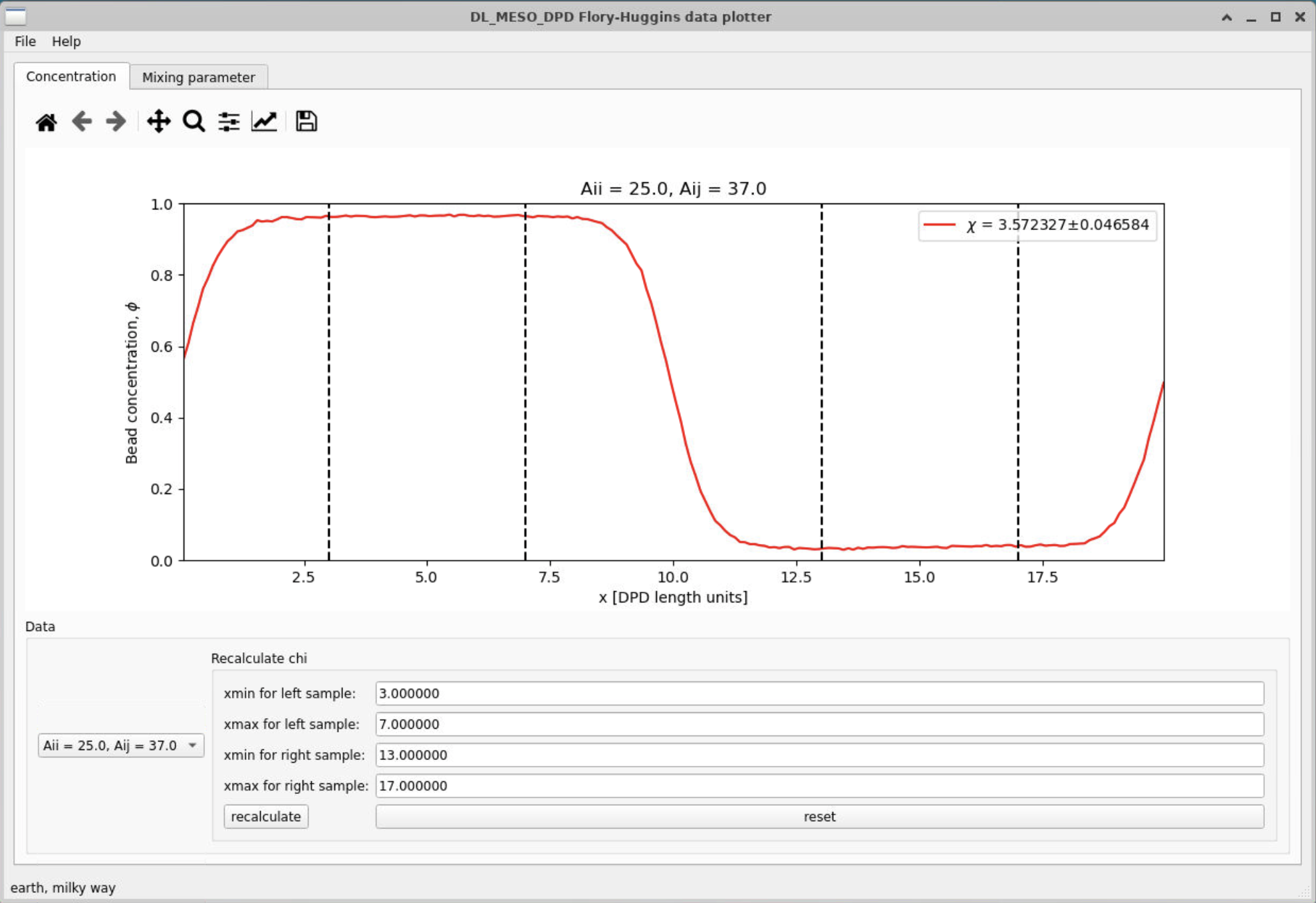
The second exercise will follow with the notebook Day9DPDTutorial1Ex2.ipynb, a link for which is provided at the end of the first notebook. One of the files in the directory is a ZIP file with DL_MESO, which you will unpack and then compile its DPD code, before using it with input files and a simulation workflow script that we have also provided. The supplied version of DL_MESO comes with a couple of additional Python scripts based on PyQt5 (a Python interface for the graphical interface framework Qt) that can be used to visualise the results of DL_MESO_DPD calculations and the simulation workflow in this exercise when not using the notebooks (e.g. on your own laptops).