Day 1-2: Introduction to Modern Fortran¶

Lecture slides are available at Fortran slides

1. Fortran comes with a rich set of intrinsic functions(see Fortran 2018 standard, chapter 16). Have a look at the following trim, adjustl, len, sin, cos, real, aimag, epsilon, huge, tiny, mod. Write a program that illustrates how they work.

2. Write a simple Fortran code that solves the quadratic equation

for any values of a,b,c using the analytical solution. The code shall handle correctly the a=0 case.

3. Consider the sum S

• Write three programs that compute the sum S. Each of them would employ a different loop construct.

• Change the previous programs so they add only the even terms. Try to use cycle.

4. Compute the sum from 3a) with your favourite loop construct. This time the sum should be computed by a function that takes as argument n and returns the sum. Try the same with a subroutine. Both the function/subroutine should be members of the program unit using contains. Refactor your previous program by putting the function/subroutine in a module that gets used by the test program.

5. Remember the Simpson’s rule to compute an definite integral of a function f(x)

with

Write a Fortran code that implements the above formula for

with a=0.0 and b=2.0 and n=10. How does the obtained value compare with the exact solution?

Change your code such way n is increased automatically until a certain precision is met.

6. Develop a vector module. It should contain:

• A vectorType with two members

  1. Integer n number of elements

  2. Real(kind=8) a(100) storage for vector

• function that computes the norm of a real vector

• Subroutine that normalizes a real vector.

• Subroutine that replaces the negative elements of a real vector by their absolute value.

• Write a main program to test your module.

7. Start with the previous exercise. Replace the storage of the vectorType members to a dynamic allocated one from a static ( hint * real(kind=8),allocatable :: a(:)*)

• add two new members to your type

  • subroutine that allocates the space for your vector, sets the member n and initializes to zero the vector

  • subroutine that releases the space used by your vector.

8. Calculate \(\pi\) using Monte Carlo. Consider a square S of side a=1.0 and the circle C with radius 1.0 and centered in the low left corner of the square S. One can estimate \(\pi\) by randomly generating points in the (x,y) in S and computing the fraction f that lands into the circle C (\(x^2+y^2<1\)) by

• Write a Fortran code that implements the above calculation of \(\pi\).

• How many points do you need to get a precision of \(10^{-3}\)?

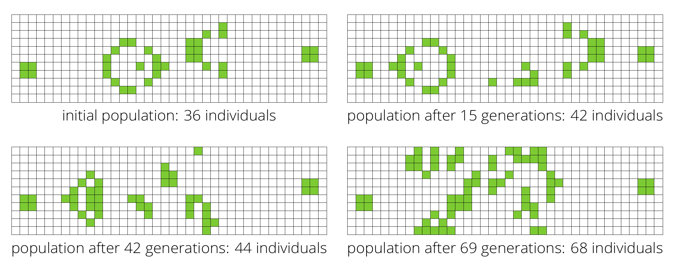
9. Conway’s Game of Life [Gardner1970] is a simple cellular automata consisting of a universe on a n by m grid. Each cell is represented by a square with two states dead or alive. Once one choses an initial condition for all the cells, by applying a set of simple rules it can determine the evolution of the system at any moment in future, see Fig. Conway’s Game of Life snapshots, n=11, m=38, ”Gosper glider gun” seed. The rules are defined as follows

1. Any cell which is alive and has fewer than two living neighbours dies. Cause of death: loneliness.

2. Any cell which is alive and has more than three living neighbours dies. Cause of death: overcrowding.

3. Any cell which is alive and has two or three living neighbours lives on to the next generation.

4. Any cell which is dead/empty and has three living neighbours becomes alive due to reproduction.

Design and build a Forran code to implement Conway’s game of life. The code shall

• Start with a random configuration of cells, then evolve them according to the above rules.

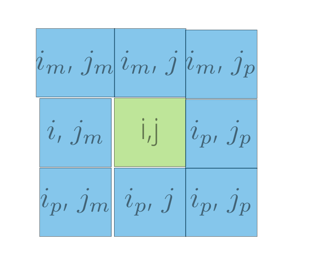
• Apply boundary conditions in both directions when you calculate the number of neighbours, see Neighbour’s update list.

• For each generation compute the total population.